EDA — Visualize Embeddings of RAG

Visualize Retrieval Augmented Generation (RAG) data using the langchain framework in conjunction with Hugging Face’s language models and embeddings and chromaDB.
Reading_time: 6 min
Tags: [UMAP,RAG,Visualization,Langchain,ChromaHuggingFaceEmbeddings]
- Introduction to RAG
- Setting Up the Environment
- Loading the Model and Vector Store
- Fetching and Preparing Data
- Calculating Distances
- Visualizing Embeddings
- Thanks for Reading!
In this article, we delve into the how we can visualize Retrieval Augmented Generation (RAG) data using the langchain framework in conjunction with Hugging Face’s language models and embeddings. We’ll explore how to leverage the HuggingFaceEmbeddings and Chroma vector store for efficient embedding and document retrieval, followed by a practical example of visualizing these embeddings to understand their distribution and relevance to a given question.
We’ll explore how to use the Hugging Face Embeddings for embedding text data and store it in chroma and then visualize it using UMAP (Uniform Manifold Approximation and Projection), a dimensionality reduction technique that helps in visualizing high-dimensional data in a more interpretable way.
 |
|---|
| Image Credits - Courtesy of Spotlight |
Introduction to RAG
RAG is a cutting-edge approach that combines the strengths of pretrained Large Language Models (LLMs) and your own data to generate responses. It retrieves documents, passes them through a sequence-to-sequence model, and then marginalizes to generate outputs. This method is particularly useful for querying specific documents or interacting with your own data in a conversational manner .
Setting Up the Environment
To begin, we’ll need to import the necessary libraries and set up our environment. We’ll use pandas for data manipulation, langchain.embeddings for handling embeddings, and langchain.vectorstores for our vector store. Introduction | 🦜️🔗 Langchain LangChain is a framework for developing applications powered by language models. It enables applications that:python.langchain.com
So do install as follow:
!pip install pandas langchain renumics-spotlight umap-learn

import pandas as pd
from langchain.embeddings import HuggingFaceEmbeddings
from langchain.vectorstores import Chroma
Loading the Model and Vector Store
Next, we’ll specify the model path for our embeddings and create instances of HuggingFaceEmbeddings and Chroma. We’ll also configure the model to use the CPU/GPU for computations and ensure embeddings are not normalized for our visualization purposes.
Before dive in we consider, you already have chroma db collection and see how we can visualize it.If no you can create one as follow:
from langchain_community.document_loaders.recursive_url_loader import RecursiveUrlLoader
from bs4 import BeautifulSoup as Soup
from langchain.vectorstores import Chroma

url = "https://www.freenews.fr/"
loader = RecursiveUrlLoader(
    url=url, max_depth=5, extractor=lambda x: Soup(x, "lxml").text
)
documents = loader.load()
text_splitter = RecursiveCharacterTextSplitter(
            chunk_size=1000, chunk_overlap=0
        )
texts = text_splitter.split_documents(documents)

modelPath = "sentence-transformers/distiluse-base-multilingual-cased-v1"

model_kwargs = {'device':'cpu'}
#encode_kwargs = {'normalize_embeddings': False}

embeddings = HuggingFaceEmbeddings(model_name=modelPath,model_kwargs=model_kwargs)

# SAVE
docs_vectorstore = Chroma.from_documents(texts, embeddings, persist_directory="./chroma_db_multilingual")
Provide the link to your chroma persist_directory below:
modelPath = "sentence-transformers/distiluse-base-multilingual-cased-v1"
model_kwargs = {'device':'cpu'}
encode_kwargs = {'normalize_embeddings': False}
embeddings_model = HuggingFaceEmbeddings(model_name=modelPath, model_kwargs=model_kwargs)
docs_vectorstore = Chroma(persist_directory="./chroma_db_multilingual", embedding_function=embeddings_model)
Fetching and Preparing Data
We’ll retrieve our data from the vector store, including metadata, documents, and embeddings. Then, we’ll create a DataFrame to organize this data and add a column to indicate whether each document contains the answer to our query.
response = docs_vectorstore.get(include=["metadatas", "documents", "embeddings"])
df = pd.DataFrame({
 "id": response["ids"],
 "source": [metadata.get("source") for metadata in response["metadatas"]],
 "page": [metadata.get("page", -1) for metadata in response["metadatas"]],
 "document": response["documents"],
 "embedding": response["embeddings"],
})
df["contains_answer"] = df["document"].apply(lambda x: "Nœud Répartition Optique)" in x)
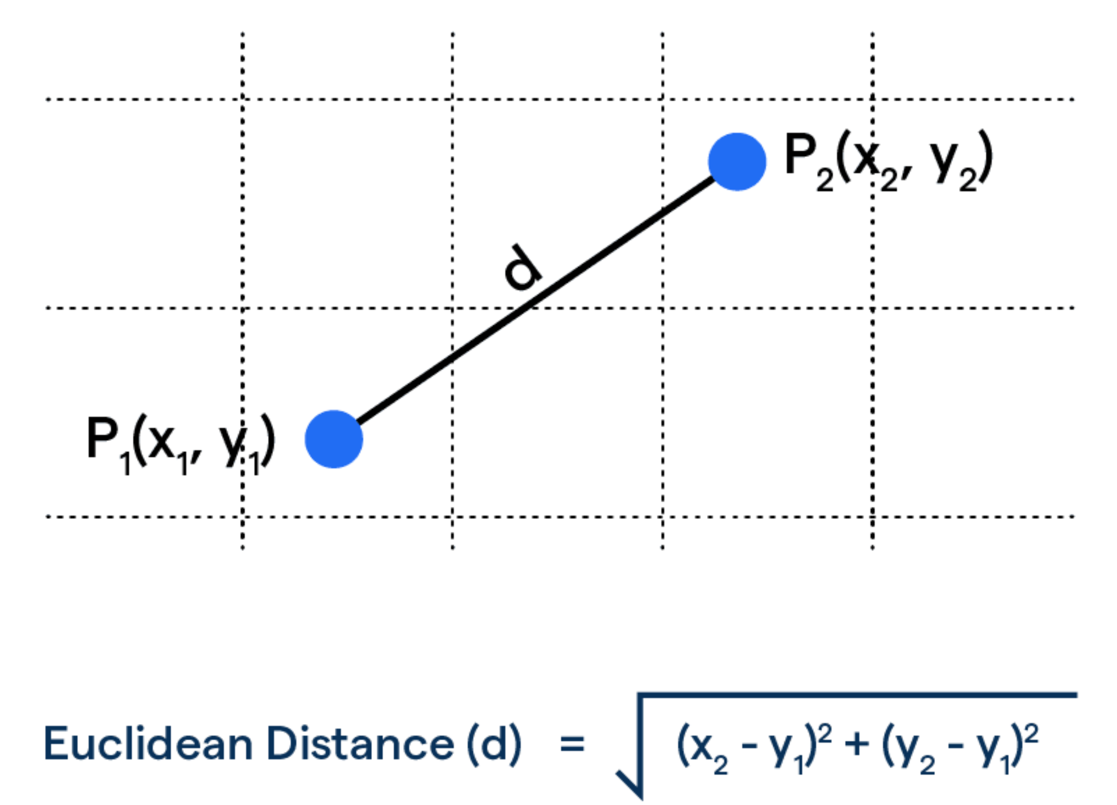
Calculating Distances
To find the closest match to our question, we calculate the Euclidean distance between the question embedding and each document embedding.
question_embedding = embeddings_model.embed_query(question)
df["dist"] = df.apply(
    lambda row: np.linalg.norm(
        np.array(row["embedding"]) - question_embedding
    ),
    axis=1,
)
Visualizing Embeddings
1. Using Spotlight
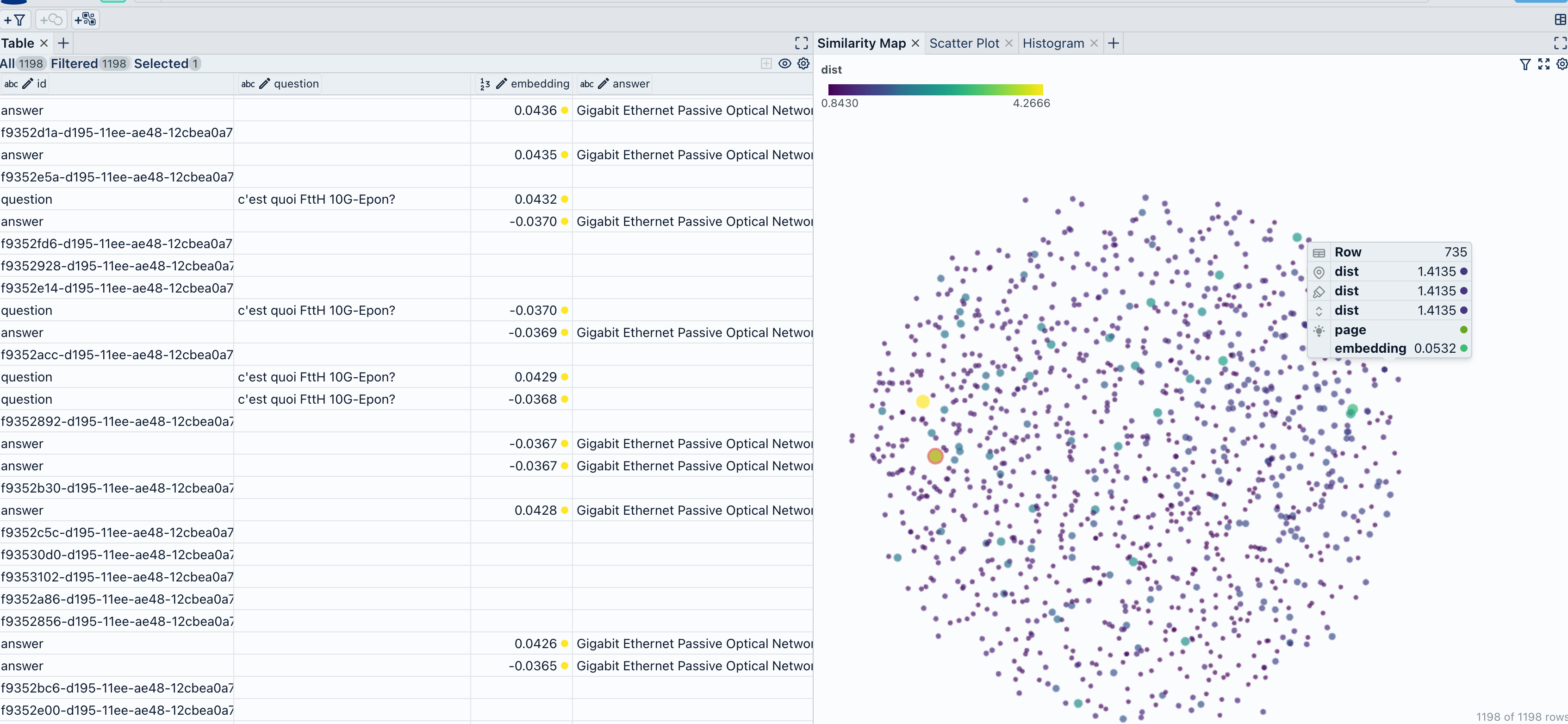
This visualization will help us understand how closely related documents are to our query and identify potential areas of improvement or further investigation.
Finally, we use the spotlight module from renumics to visualize the data. This step is crucial for understanding the distribution of documents in relation to the question and the model’s response. GitHub - Interactively explore unstructured datasets from your dataframe-Interactively explore unstructured datasets from your dataframe
from renumics import spotlight
spotlight.show(df)
Notebook-Renumics/rag-demo.Retrieval-Augmented Generation Assistant Demo
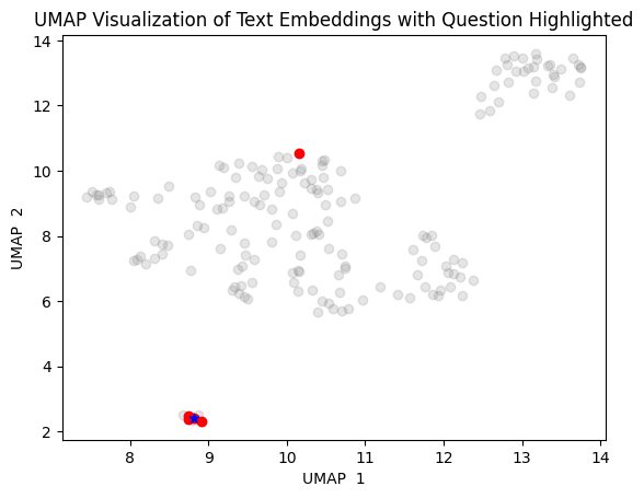
2. Using UMAP
import umap
# Find the  5 closest vectors
closest_vectors_indices = df.nsmallest(5, 'dist')['id'].values

# Prepare the embeddings for UMAP
embeddings = np.array([np.array(x) for x in df["embedding"]])

# Reduce dimensionality with UMAP
reducer = umap.UMAP()
embedding_reduced = reducer.fit_transform(embeddings)

# Plot the reduced embeddings
plt.scatter(embedding_reduced[:,  0], embedding_reduced[:,  1], c='gray', alpha=0.2)

# Highlight the question embedding and the  5 closest vectors
plt.scatter(embedding_reduced[df["id"].isin(closest_vectors_indices),  0], embedding_reduced[df["id"].isin(closest_vectors_indices),  1], c='red', alpha=1)
plt.scatter(embedding_reduced[df["id"] == df[df["dist"] == df["dist"].min()]["id"].values[0],  0], embedding_reduced[df["id"] == df[df["dist"] == df["dist"].min()]["id"].values[0],  1], c='blue', alpha=1, marker='*')

# Add labels and title
plt.title("UMAP Visualization of Text Embeddings with Question Highlighted")
plt.xlabel("UMAP  1")
plt.ylabel("UMAP  2")
plt.show()
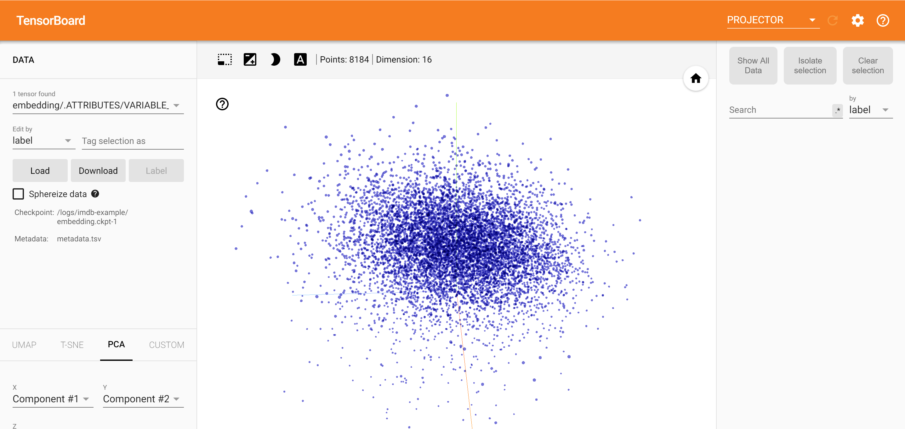
3. Using Tensorboard
Another effective way to visualize embeddings, especially useful for gaining insights into word embeddings and the relationships between them, is by using TensorBoard. TensorBoard is a tool that allows for the visualization of machine learning models and their metrics, including word embeddings, in a user-friendly interface. It can be particularly beneficial when you want to explore the semantic similarities and relationships between words in your embeddings.
Setting Up TensorBoard
First, ensure you have TensorBoard installed. You can install it using pip:
pip install tensorboard
Visualizing Word Embeddings with TensorBoard
To visualize word embeddings using TensorBoard, you’ll typically need to convert your embeddings into a format that TensorBoard can understand. This often involves creating a metadata file that maps words to their embeddings and then using TensorBoard’s Projector to visualize these embeddings. Get started with TensorBoard | TensorFlow
Here’s a simplified step-by-step guide on how to do this:
Prepare Your Embeddings: Ensure your embeddings are in a suitable format. For TensorBoard, you might need to convert your embeddings into a
.tsv(Tab-Separated Values) file where each line contains a word and its corresponding embedding vector.Create a Metadata File: Alongside your embeddings file, create a metadata file that maps each word to its index in the embeddings file. This file is also in
.tsvformat.Use TensorBoard’s Projector: — Start TensorBoard by running
tensorboard — logdir=path/to/your/logsin your terminal. — In your web browser, navigate to the TensorBoard interface (usually atlocalhost:6006). — Go to theProjectortab. — Click onLoadunder theEmbeddingssection. — Upload your embeddings file and metadata file.Explore Your Embeddings: — Once your embeddings are loaded, you can explore them in various ways, such as through a 2D or 3D scatter plot, where each point represents a word and its position is determined by its embedding vector. — You can also use the
Wordsearch bar to find specific words and see how they are positioned relative to others in the embedding space.
-Semantic Similarity: TensorBoard makes it easier to visually inspect the semantic relationships between words by examining their positions in the embedding space.
- Ease of Use: The user-friendly interface of TensorBoard allows for intuitive exploration of embeddings without the need for complex code.
- Insight into Model Performance: Beyond visualizing embeddings, TensorBoard can also be used to track model metrics, network weight distributions, and other performance indicators, providing a comprehensive toolkit for monitoring and understanding your models.
Conclusion
Visualizing RAG data provides valuable insights into the model’s decision-making process, helping us understand how it selects and interprets information from external documents.By visualizing RAG data, we gain valuable insights into the relationships between documents and our queries. This technique not only aids in understanding the performance of our RAG system but also guides us in refining models and datasets for better accuracy and relevance.
Thanks for Reading!